Dispersion of a triangular lattice

Contents

Define the model and compute

spec = sw_egrid(spinwave(sw_model('triAF',1),{[0 0 0] [1 1 0] 501}));

Warning: To make the Hamiltonian positive definite, a small omega_tol value was
added to its diagonal! 

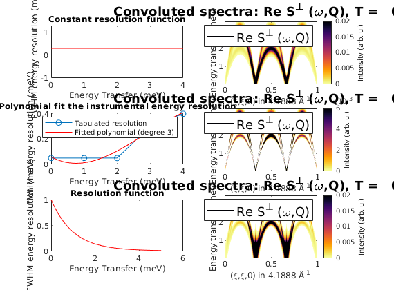
constant resolution

figure;

% plot the constant resolution value
dE = 0.3;
subplot(3,2,1)
plot([0 4],[dE dE],'r-')
title('Constant resolution function')
xlabel('Energy Transfer (meV)')
ylabel('FWHM energy resolution (meV)')

% apply constant resolution on the simulation
subplot(3,2,2)
spec = sw_instrument(spec,'dE',0.3);
sw_plotspec(spec,'mode','color');


% fit and plot tabulated resoltuion values and apply to the simulation
EN = [0       1   2    3   4]; % meV
dE = [0.05 0.05 0.05 0.3 0.4]; % meV
R  = [EN' dE'];

subplot(3,2,3)
spec = sw_instrument(spec,'dE',R,'polDeg',3,'plot',true);

subplot(3,2,4)
sw_plotspec(spec,'mode','color');

% resolution is defined by user provided function (anonymous or .m file)
a = 0.01;
b = 1.0;
resFun = @(x)a+b*exp(-x);

% plot the user defined resolution function
xVal = linspace(0,5,501);
subplot(3,2,5)
plot(xVal,resFun(xVal),'r-')
title('Resolution function')
xlabel('Energy Transfer (meV)')
ylabel('FWHM energy resolution (meV)')

% apply the function to the simulation
subplot(3,2,6)
spec = sw_instrument(spec,'dE',resFun);
sw_plotspec(spec,'mode','color');

Published with MATLAB® R2018b