Frustrated J1-J2 AFM chain

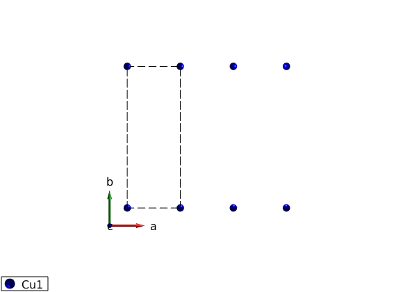
Crystal structure, shortest bond along a-axis, Cu+ magnetic atoms with S=1 spin.

Define the lattice
Couplings
Magnetic structure is a helix
Direct input
We optimise the helix pitch angle
Spin wave spectrum

Define the lattice

J1J2chain = spinw;
J1J2chain.genlattice('lat_const',[3 8 10],'angled',[90 90 90],'spgr',0);
J1J2chain.addatom('r',[0 0 0],'S',1,'label','Cu1','color','blue');
disp('Magnetic lattice:')
J1J2chain.table('atom')
plot(J1J2chain,'range',[3 1 1],'zoom',0.5)

Magnetic lattice:

ans =

  1×4 table

    matom    idx    S        pos    
    _____    ___    _    ___________

    'Cu1'     1     1    0    0    0

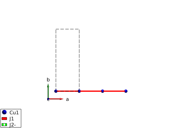
Couplings

First and second neighbor antiferromagnetic couplings. If the name of the matrix ends with '-' the bond is plotted with dashed line.

J1J2chain.gencoupling('maxDistance',7);
disp('Bonds:')
J1J2chain.table('bond',[])

J1J2chain.addmatrix('label','J1', 'value',-1,'color','r');
J1J2chain.addmatrix('label','J2-','value', 2,'color','g');

J1J2chain.addcoupling('mat','J1','bond',1);
J1J2chain.addcoupling('mat','J2-','bond',2);
plot(J1J2chain,'range',[3 0.9 0.9],'bondMode','line','bondLinewidth0',3)

Bonds:

ans =

  2×10 table

    idx    subidx        dl             dr         length    matom1    idx1    matom2    idx2        matrix    
    ___    ______    ___________    ___________    ______    ______    ____    ______    ____    ______________

     1       1       1    0    0    1    0    0      3       'Cu1'      1      'Cu1'      1      ''    ''    ''
     2       1       2    0    0    2    0    0      6       'Cu1'      1      'Cu1'      1      ''    ''    ''

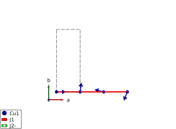
Magnetic structure is a helix

We use two different methods to define the ground state magnetic structure:

Direct input

If we would know the exact solution of the spin Hamiltonian we can input that, assuming a helix with the following parameters:

magnetic ordering wave vector k = (1/4 0 0)
spins lying in arbitrary plane, first spin S = (1 0 0)
normal to the plane of the spin helix has to be perpendicular to S, we choose it n = (0 0 1)
we won't use a magnetic supercell, not necessary

J1J2chain.genmagstr('mode','helical', 'k',[0.25 0 0], 'n',[0 0 1], 'S',[1; 0; 0], 'nExt',[1 1 1])
disp('Magnetic structure:')
J1J2chain.table('mag')
disp('Ground state energy before optimization:')
J1J2chain.energy

plot(J1J2chain,'range',[3 0.9 0.9])

Magnetic structure:

ans =

  1×8 table

    num    matom    idx    S     realFhat       imagFhat          pos               kvect        
    ___    _____    ___    _    ___________    ___________    ___________    ____________________

     1     'Cu1'     1     1    1    0    0    0    1    0    0    0    0    0.25       0       0

Ground state energy before optimization:
Ground state energy: -2.000 meV/spin.

We optimise the helix pitch angle

We are unsure about the right pitch angle of the helix, thus we want to calculate it. The sw.optmagstr() is able to determine the magnetic ground state. It uses a constraint function (@gm_planar in this case) to reduce the number of paramteres that has to be optimised. It works well if the number of free parameters are low. we will find the the right k-vector is 0.2301.

%     Phi1 k_x k_y k_z nTheta nPhi
x1 = [0      0   0   0      0    0];
x2 = [0    1/2   0   0      0    0];
optRes = J1J2chain.optmagstr('func',@gm_planar,'xmin',x1,'xmax',x2,'nRun',10);
disp('Ground state energy after optimization')
J1J2chain.energy
disp('Optimized magnetic structure:')
J1J2chain.table('mag')

plot(J1J2chain,'range',[3 0.9 0.9],'bondMode','line','bondLineWidth0',3)

Ground state energy after optimization
Ground state energy: -2.062 meV/spin.
Optimized magnetic structure:

ans =

  1×8 table

    num    matom    idx    S     realFhat       imagFhat          pos                    kvect            
    ___    _____    ___    _    ___________    ___________    ___________    _____________________________

     1     'Cu1'     1     1    1    0    0    0    1    0    0    0    0    0.23005          0          0

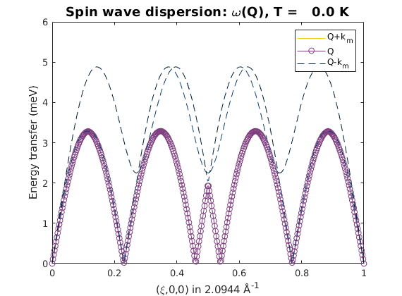
Spin wave spectrum

We calculate the spin wave spectrum, the code automatically uses the method that enables the spin wave calculation of incommensurate structures withouth creating a magnetic supercell. There are three spin wave modes, these are omega(Q), omega(Q+/-k). The two shifted ones are due to the incommensurate structure.

J1J2spec= J1J2chain.spinwave({[0 0 0] [1 0 0] 400}, 'hermit',false);
J1J2spec = sw_neutron(J1J2spec);
J1J2spec = sw_egrid(J1J2spec, 'Evect',linspace(0,6.5,100));
figure
sw_plotspec(J1J2spec, 'mode',1,'colorbar',false)
axis([0 1 0 6])

Warning: Eigenvectors of defective eigenvalues cannot be orthogonalised at some
q-point!

Written by
Bjorn Fak & Sandor Toth
06-Jun-2014, 06-Feb-2017

Tutorial 3