spinw.spinwavesym method

Syntax

spectra = spinwavesym(obj,Name,Value)

Description

spectra = spinwavesym(obj,Name,Value) calculates symbolic spin wave dispersion as a function of \(Q\). The function can deal with arbitrary magnetic structure and magnetic interactions as well as single ion anisotropy and magnetic field. Biquadratic exchange interactions are also implemented, however only for \(k=0\) magnetic structures.

If the magnetic propagation vector is non-integer, the dispersion is calculated using a coordinate system rotating from cell to cell. In this case the Hamiltonian has to fulfill this extra rotational symmetry.

The method works for incommensurate structures, however the calculated omega dispersion does not contain the \(\omega(\mathbf{k}\pm \mathbf{k}_m)\) terms that has to be added manually.

The method for matrix diagonalization is according to R.M. White, PR 139 (1965) A450. The non-Hermitian g*H matrix will be diagonalised.

Examples

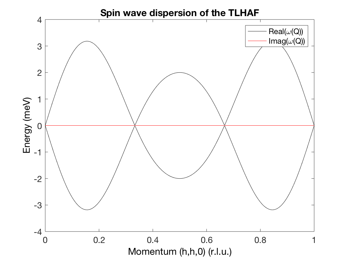
The first section of the example calculates the symbolic spin wave spectrum. Unfortunatelly the symbolic expression needs manipulations to bring it to readable form. To check the solution, the second section converts the symbolic expression into a numerical vector and the third section plots the real and imaginary part of the solution.

tri = sw_model('triAF',1)
tri.symbolic(true)
tri.genmagstr('mode','direct','k',[1/3 1/3 0],'S',[1 0 0])
symSpec = tri.spinwave
pretty(symSpec.omega)

Output

/ -#1 \
|     |
\  #1 /
where
         sqrt(2) J_1 exp(-4 pi #2) sqrt(exp(2 pi #2) + #6 + #5 + exp(4 pi #2) 3 + #4 + #3 + exp(6 pi #2)) sqrt(- exp(2 pi #2) - #6 - #5 + exp(4 pi #2) 6 - #4 - #3 - exp(6 pi #2))
   #1 == -------------------------------------------------------------------------------------------------------------------------------------------------------------------------
                                                                                             2
   #2 == h 1i + k 1i
   #3 == exp(2 pi (h 3i + k 2i))
   #4 == exp(2 pi (h 2i + k 3i))
   #5 == exp(2 pi (h 2i + k 1i))
   #6 == exp(2 pi (h 1i + k 2i))

J_1 = 1
h = linspace(0,1,500)
k = h
omega = eval(symSpec.omega)
p1 = plot(h,real(omega(1,:)),'k-')
hold on
plot(h,real(omega(2,:)),'k-')
p2 = plot(h,imag(omega(1,:)),'r-')
plot(h,imag(omega(2,:)),'r-')
xlabel('Momentum (h,h,0) (r.l.u.)')
ylabel('Energy (meV)')
legend([p1 p2],'Real(\omega(Q))','Imag(\omega(Q))')
title('Spin wave dispersion of the TLHAF')

title('Spin wave dispersion of the TLHAF')

Input Arguments

obj: spinw object.

Name-Value Pair Arguments

'hkl'

Symbolic definition of \(Q\) vector. Default is the general \(Q\) point:

hkl = [sym('h') sym('k') sym('l')]

'eig'

If true the symbolic Hamiltonian is diagonalised symbolically. For large matrices (many magnetic atom per unit cell) this might be impossible. Set eig to false to output only the quadratic Hamiltonian. Default is true.

'vect'

If true the eigenvectors are also calculated. Default is false.

'tol'

Tolerance of the incommensurability of the magnetic ordering wavevector. Deviations from integer values of the ordering wavevector smaller than the tolerance are considered to be commensurate. Default value is \(10^{-4}\).

'norm'

Whether to produce the normalized symbolic eigenvectors. It can be impossible for large matrices, in that case set it to false. Default is true.

'fid'

Defines whether to provide text output. The default value is determined by the fid preference stored in swpref. The possible values are:

0 No text output is generated.
1 Text output in the MATLAB Command Window.
fid File ID provided by the fopen command, the output is written into the opened file stream.

'title'

Gives a title string to the simulation that is saved in the output.

Output Arguments

spectra

Structure, with the following fields: